Clouds from equations
vizz draws point clouds. Most of them come from a scanner, a camera or a file — and 72 of them come from mathematics, with 22 more that are still running while you watch.
Every picture on this page was drawn by the app's own code, from the same functions that fill a slot when you pick one from the menu, and through the same renderer that puts it on screen. Nothing here is an artist's impression of what a generator makes.
To use one: open the clouds section of the panel and pick from
generate…, or start vizz with --cloud gen:thomas. A made cloud
takes the next free slot and behaves exactly as a scanned one does: chosen by
name, crossed to with a scene change, captured by a preset, lit, and remade the
next time you launch. The ones with knobs take them after a ? —
gen:torus-knot?p=2;q=5. The live ones run in the live slot:
--live-cloud sim:fluid, or simulate… beside receive.
Where these came from. Almost none of it is ours. Each entry says whose work it is, and links to somewhere to read about it where there is somewhere worth sending you. If we have credited something wrongly, that is a bug like any other — please tell us.
And the rest of it. Clouds are the part of vizz with the longest bibliography, but the shader's own shapes, the pattern stack, the colour, the light, the beat detection and the passes at the end all came from somewhere too. Those are below the catalogue, and everything on the page is in one list at the foot of it.
flows
Differential equations, integrated from one point on the attractor and recorded in time order. Consecutive points are consecutive moments, which is what makes the cloud crawl along itself rather than shimmer.
Thomas
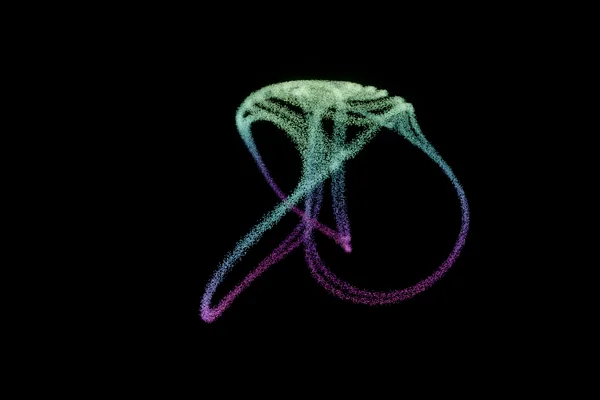
gen:thomas
Thomas' cyclically symmetric attractor — three sines; a knot of ribbons round the diagonal
Halvorsen
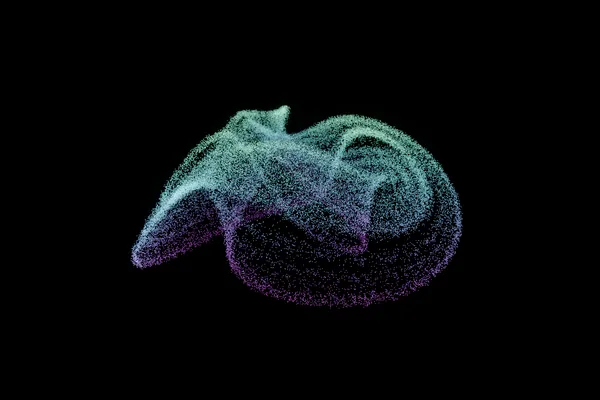
gen:halvorsen
Halvorsen's attractor — three lobes, cyclically symmetric; sheets folding into each other
Arne Dehli Halvorsen’s cyclically symmetric system, as catalogued by Sprott
Dadras
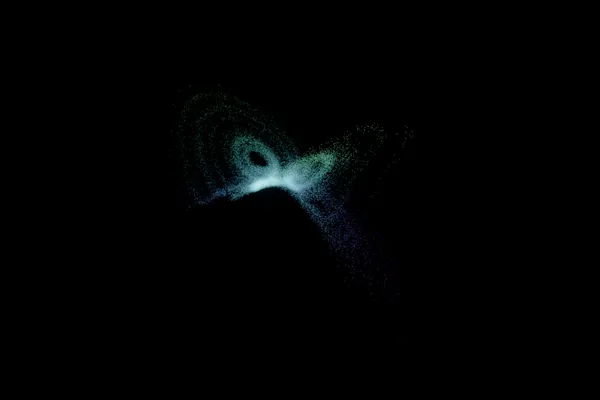
gen:dadras
Dadras' tri-scroll — three rolled sheets joined by a spine
Sara Dadras & Hamid Reza Momeni, Physics Letters A 373 (2009)
Rössler
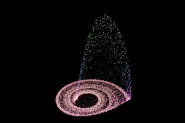
gen:rossler
Rössler's funnel — a flat spiral that lifts and folds back on itself
Otto Rössler, “An equation for continuous chaos”, Physics Letters A 57 (1976)
Four-wing
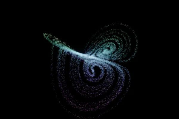
gen:four-wing
the four-wing attractor — four lobes off a saddle
Wang, Sun & van Wyk, the four-wing system (2009)
Chen
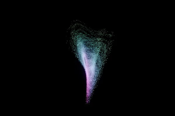
gen:chen
Chen's system — Lorenz's cousin, wider and more tangled
Sprott B
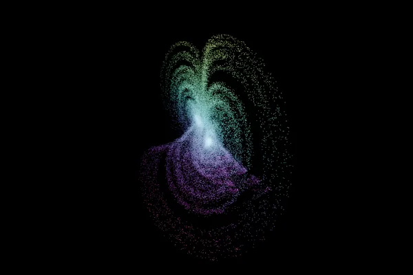
gen:sprott-b
Sprott's case B — two quadratic terms, and chaos
Julien Clinton Sprott, “Some simple chaotic flows”, Phys. Rev. E 50 (1994) — case B
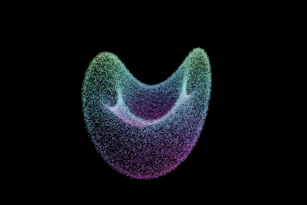
Nosé–Hoover
gen:nose-hoover
the Nosé–Hoover oscillator — a thermostatted particle wandering a sea of tori and chaos
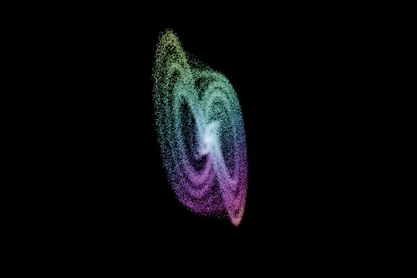
Arneodo
gen:arneodo
Arneodo's attractor — a jerk system with one cubic term
Alain Arnéodo, Pierre Coullet & Charles Tresser (1981)
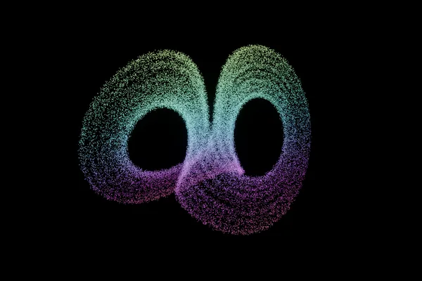
Burke–Shaw
gen:burke-shaw
Burke–Shaw — two scrolls with the symmetry of a propeller
Bill Burke & Robert Shaw (1981)
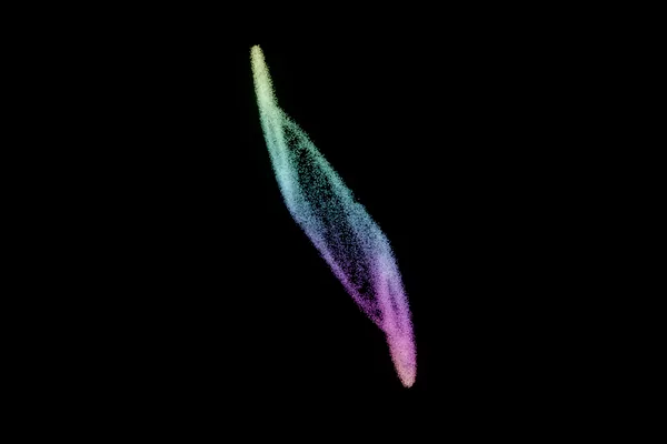
Chua
gen:chua
Chua's circuit — the double scroll, from a real circuit with a nonlinear diode
Leon Chua (1983); Matsumoto, Chua & Komuro, IEEE Trans. Circuits and Systems 32 (1985)
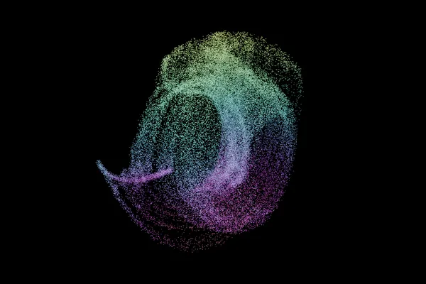
Hadley
gen:hadley
the Hadley circulation — Lorenz's 1984 atmosphere in three variables
Edward Lorenz, “Irregularity: a fundamental property of the atmosphere”, Tellus 36A (1984)
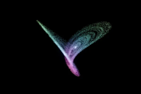
Rucklidge
gen:rucklidge
Rucklidge's convection model — a tall, folded ribbon
Alastair Rucklidge, “Chaos in models of double convection”, J. Fluid Mech. 237 (1992)
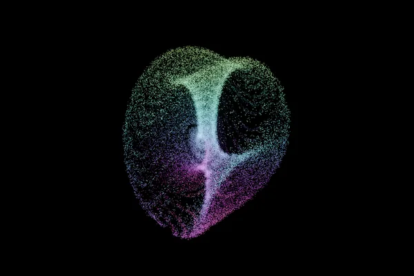
three-scroll
gen:three-scroll
the three-scroll unified system — three scrolls in one fast flow
The three-scroll unified chaotic system; Dequan Li, Physics Letters A 372 (2008)
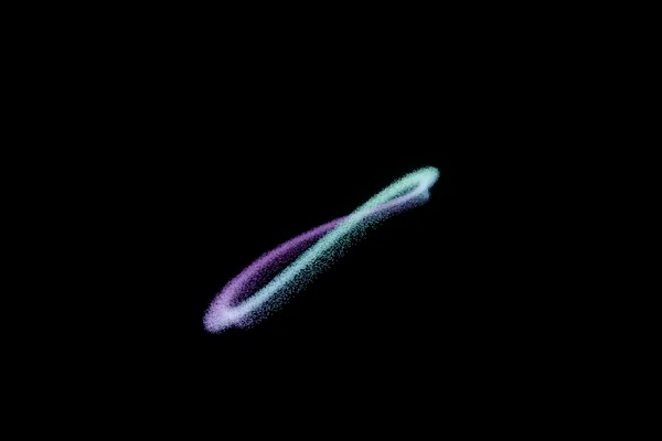
Rabinovich–Fabrikant
gen:rabinovich
Rabinovich–Fabrikant — leaves and ribbons, from plasma physics
Mikhail Rabinovich & Anatoly Fabrikant, Sov. Phys. JETP 50 (1979)
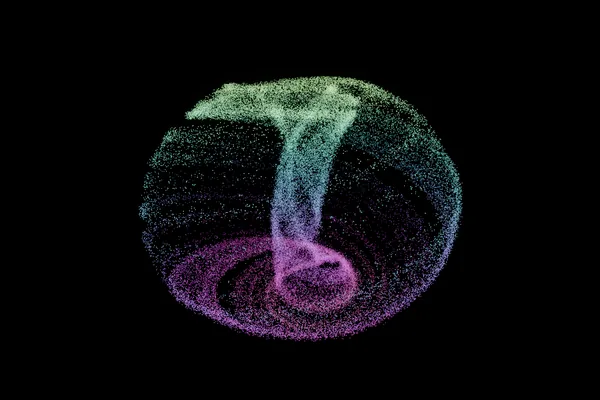
Aizawa
gen:aizawa
Aizawa's attractor — a rotating sphere with a spindle driven through its poles
Yoji Aizawa & Tatsuo Uezu (1982), as catalogued by Chaoscope
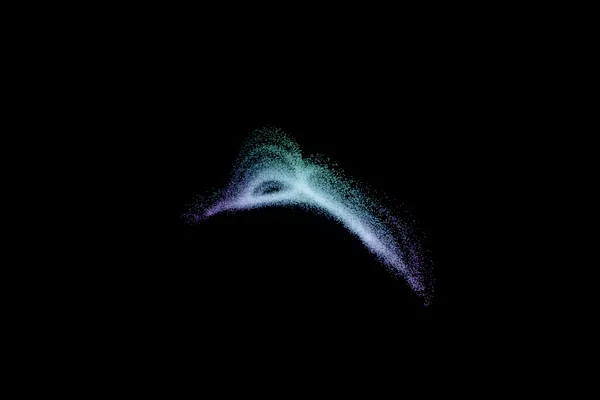
Newton–Leipnik
gen:newton-leipnik
Newton–Leipnik — a tumbling rigid body, and two attractors in one system
Tim Newton & Roy Leipnik, “Double strange attractors in rigid body motion”, SIAM J. Appl. Math. 41 (1981)
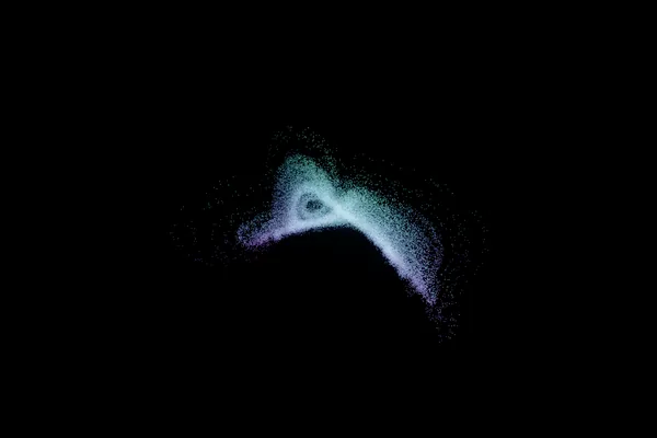
Sakarya
gen:sakarya
the Sakarya system — two lobes crossing at an angle, like a bow tie in wire
The Sakarya system (2010)
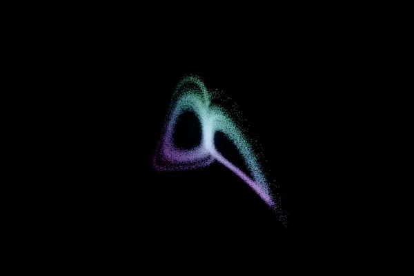
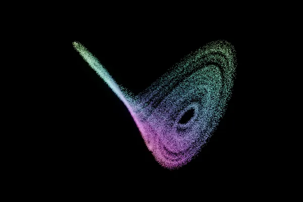
Rikitake
gen:rikitake
the Rikitake dynamo — why the Earth's magnetic field reverses, and never on schedule
Shimizu–Morioka
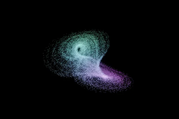
gen:shimizu-morioka
Shimizu–Morioka — the butterfly's simplest relative, two wings and one quadratic term
Tsutomu Shimizu & Nobuo Morioka, Physics Letters A 76 (1980)
finance
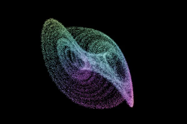
gen:finance
the finance system — interest rate, investment demand and price index, refusing to settle
Junhai Ma & Yushu Chen, Applied Mathematics and Mechanics 22 (2001)
Coullet
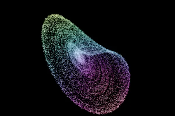
gen:coullet
Coullet's jerk system — one variable's third derivative, with a cubic pull
Pierre Coullet, Charles Tresser & Alain Arnéodo (1979) — a jerk system
Genesio–Tesi
gen:genesio-tesi
Genesio–Tesi — the other classic jerk system, square rather than cubic
Roberto Genesio & Alberto Tesi, Automatica 28 (1992)
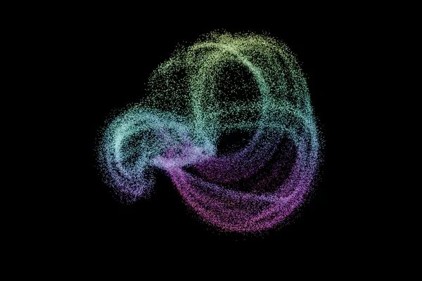
Lorenz-96
gen:lorenz96
Lorenz's toy atmosphere: a ring of variables advecting each other; the test bed every weather forecasting scheme meets first
knobs size how many round the ring (4 to 40, default 5)
forcing how hard it is driven; 8 is the chaotic one (0 to 20, default 8)
Edward Lorenz, “Predictability: a problem partly solved”, ECMWF Seminar on Predictability (1996)
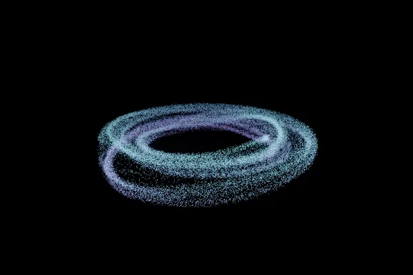
Duffing
gen:duffing
a mass in a double well, shaken — drawn on the cylinder of the forcing phase, so once round the tube is one period
knobs drive how hard it is shaken (0 to 2, default 0.5)
Georg Duffing (1918); the chaotic forced case is Ueda’s (1979)
maps
Iterated rather than integrated: a rule applied over and over to a point in a plane, lifted into depth by delay embedding — Takens' theorem says a delayed coordinate unfolds the dynamics rather than merely decorating them.
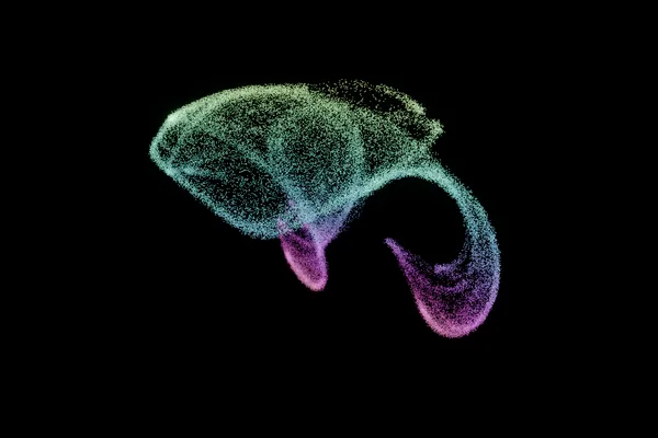
Clifford
gen:clifford
Pickover's Clifford map, lifted into depth by its own previous step
Clifford Pickover, Computers, Pattern, Chaos and Beauty (1990)
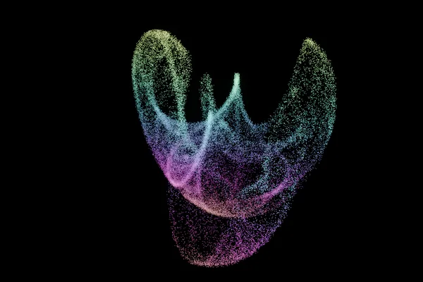
de Jong
gen:dejong
the Peter de Jong map of 1987, lifted the same way
Peter de Jong, in A. K. Dewdney’s Computer Recreations, Scientific American (1987)
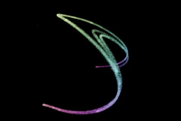
Hénon
gen:henon
the Hénon map — the first attractor anyone drew that was plainly a fractal
Michel Hénon, “A two-dimensional mapping with a strange attractor”, Comm. Math. Phys. 50 (1976)
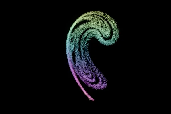
Ikeda
gen:ikeda
the Ikeda map — light in a ring cavity, with a hook in the attractor nothing else here has
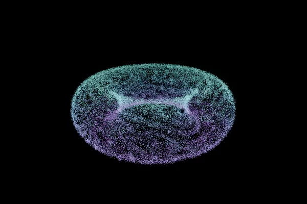
standard map
gen:standard
Chirikov's standard map on its torus — islands that close, and one orbit that never does
knobs k how hard each turn is kicked; at 0.9716 the last ring across the picture breaks (0 to 4, default 0.971635)
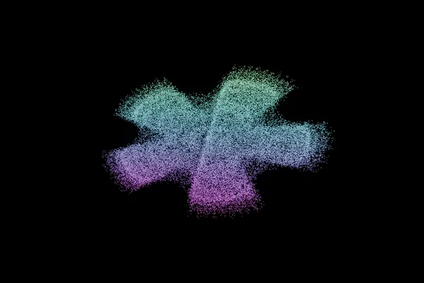
Gumowski–Mira
gen:gumowski
from a study of particle beams at CERN — moths and mandalas that change completely in the third decimal place
knobs mu the one number; try small changes (-1 to 1, default -0.801)
Igor Gumowski & Christian Mira, CERN (1980)
searched
Nobody chose these. Thirty coefficients are drawn at random and the result is kept only if it is chaotic, which about one draw in a few hundred is. The seed is the whole parameter, so the same seed is the same attractor on every machine.
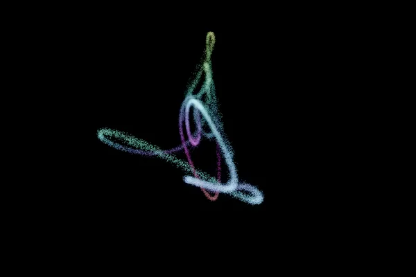
quadratic
gen:quadratic
Sprott's search: random quadratic maps until one is chaotic — a new attractor every roll
knobs seed which search; the same seed is the same attractor on every machine (any whole number, default 1)
Julien Clinton Sprott, Strange Attractors: Creating Patterns in Chaos (1993)
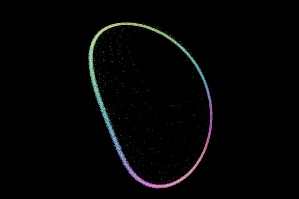
quadratic flow
gen:quadratic-flow
the same search with an integrator inside: random quadratic flows until one is chaotic — smooth ribbons where the map gives dust
knobs seed which search; the same seed is the same attractor on every machine (any whole number, default 1)
The same search over quadratic flows; Sprott, “Some simple chaotic flows”, Phys. Rev. E 50 (1994)
surfaces
Swept in scan order over two parameters, so the cloud reads as a surface rather than a fog.
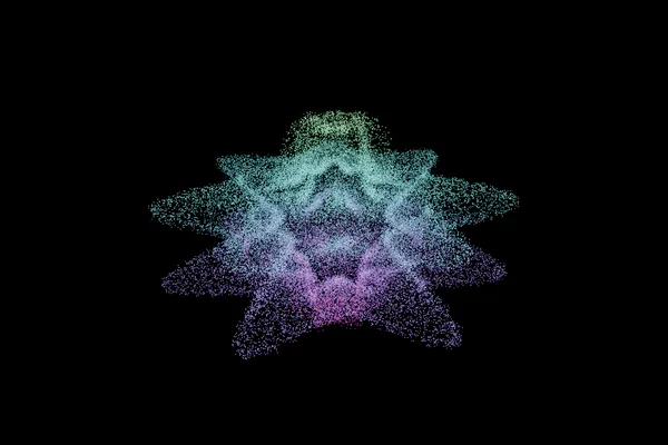
supershape
gen:supershape
Gielis' superformula as a solid — a seven-fold flower
knobs m fold: how many times round the symmetry repeats (1 to 16, default 7)
n1 overall roundness — small pinches, large bloats (0.1 to 10, default 2)
n2 the cosine exponent (0.1 to 20, default 8)
n3 the sine exponent (0.1 to 20, default 4)
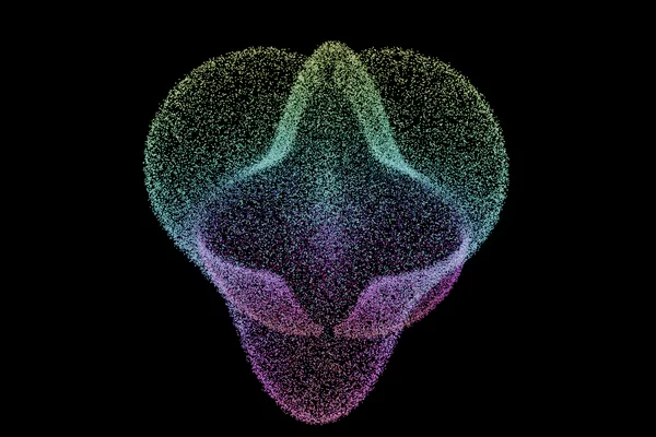
harmonic
gen:harmonic
a sphere rippled by a spherical harmonic
knobs round waves round the equator (1 to 8, default 3)
up waves pole to pole (1 to 8, default 2)
A sphere modulated by a spherical harmonic; the classical functions of Laplace (1782)
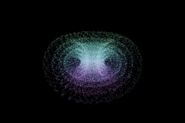
Hopf
gen:hopf
the Hopf fibration — nested tori of linked circles, projected from the 3-sphere
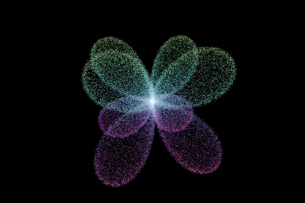
orbital
gen:orbital
a real spherical harmonic as a balloon — the shape a textbook draws for an atomic orbital
knobs l degree: how many nodal lines in all (0 to 8, default 3)
m order: how many of them run through the poles; negative turns the lobes (-8 to 8, default 2)
The real spherical harmonics, as a chemistry textbook draws an atomic orbital
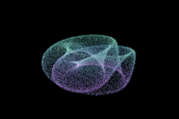
Klein bottle
gen:klein
the figure-eight immersion — a surface with no inside, and the crossing that three dimensions force on it
knobs girth how fat the tube is against the ring (0.5 to 5, default 2)
Felix Klein (1882); the figure-eight immersion is the standard one
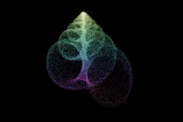
seashell
gen:seashell
a coiled shell as Raup described every one: a curve swept along a growing helico-spiral, placed by three numbers — how fast it grows, how far from the axis, how fast it slides down it — with growth ridges round the lip
knobs W how much the curve grows in one whorl (1.1 to 100, default 1.6)
D the inner edge's distance from the axis, as a share of the outer's: 0 is a solid column, near 1 an open coil (0 to 0.9, default 0.05)
T how fast it slides down the axis: 0 is a flat ammonite, 3 a tall turret (0 to 6, default 2.6)
whorls turns of the spiral (1 to 16, default 8)
ribs growth ridges per radian of turn (0 to 80, default 22)
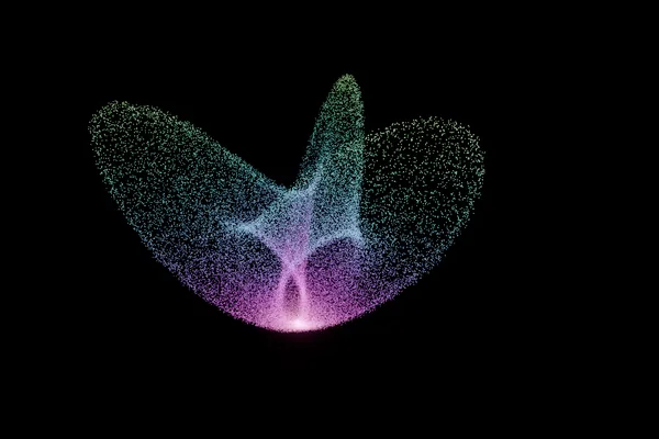
Boy's surface
gen:boy
the projective plane immersed without a boundary — three-fold symmetric, and thought impossible until 1901
Werner Boy (1901); this parametrisation is François Apéry’s (1986)
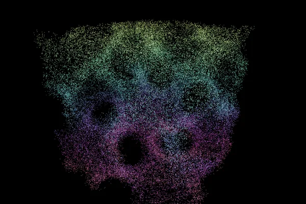
gyroid
gen:gyroid
a triply periodic minimal surface — two labyrinths that fill space and never touch; also Schwarz's P and D
knobs kind gyroid, schwarz or diamond (text, default gyroid)
cells how many periods across the box; more is denser and harder to read (1 to 6, default 1.5)
level 0 is the minimal surface; either side of it thickens one labyrinth and thins the other (-1.5 to 1.5, default 0)
thickness how thick to draw the wall (0.01 to 0.4, default 0.07)
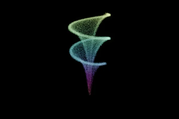
Dini
gen:dini
a pseudosphere dragged along a helix — constant negative curvature, everywhere the same
knobs twist how fast the horn climbs (0 to 1, default 0.2)
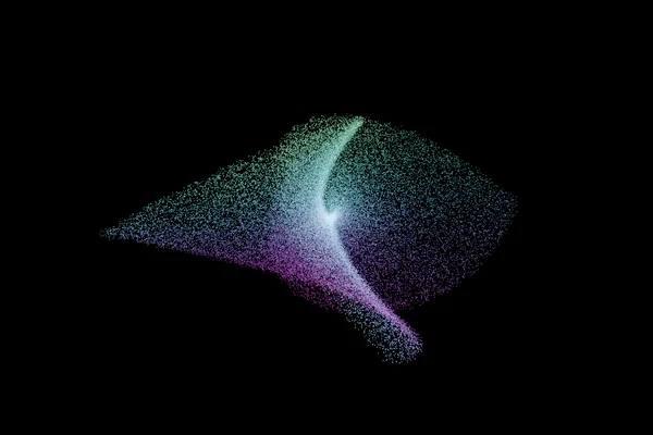
Enneper
gen:enneper
a minimal surface from 1864 that runs through itself twice, which is exactly the interesting part
curves
Traced along a curve and thickened into a tube, in order, so the crawl runs along the curve.
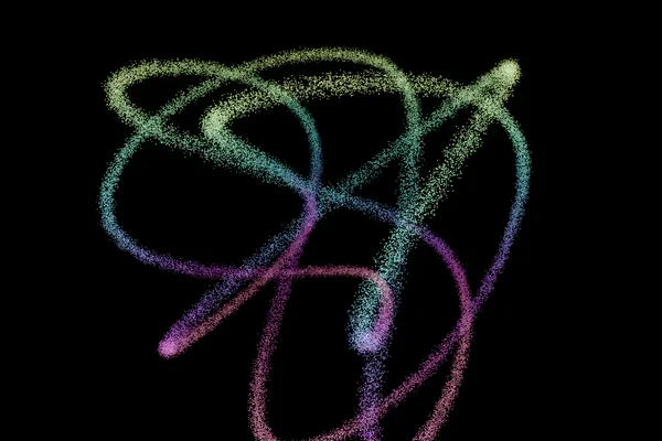
Lissajous
gen:lissajous
a 3:4:7 Lissajous knot, as a tube
knobs a frequency on x (1 to 9, default 3)
b frequency on y (1 to 9, default 4)
c frequency on z (1 to 12, default 7)
Jules Antoine Lissajous (1857); the knotted case is Bogle, Hearst, Jones & Stoilov (1994)
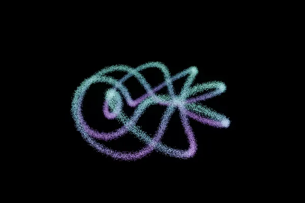
torus knot
gen:torus-knot
a (3,7) torus knot — three times round, seven times through
knobs p times round the axis (1 to 9, default 3)
q times through the hole (1 to 12, default 7)
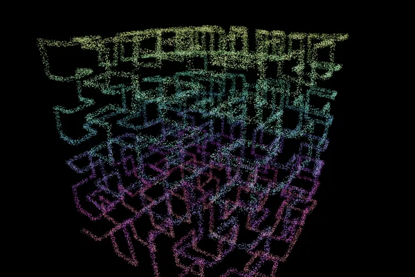
Hilbert curve
gen:hilbert
one unbroken line through every cell of a cube — the cloud crawls along a curve that fills space
knobs order how many times the curve folds into itself (1 to 5, default 3)
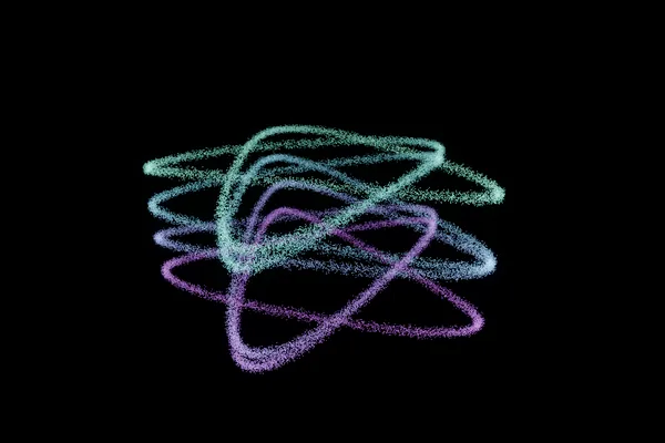
spirograph
gen:spirograph
the curve a pen traces through a hole in a wheel rolling inside another, given a slow rise so it coils
knobs R the big wheel (1 to 20, default 5)
r the small wheel; the ratio decides the petals (0.2 to 19, default 3)
pen how far the pen sits from the roller's centre (0.1 to 20, default 5)
wave how many times it climbs and falls (0 to 8, default 1)
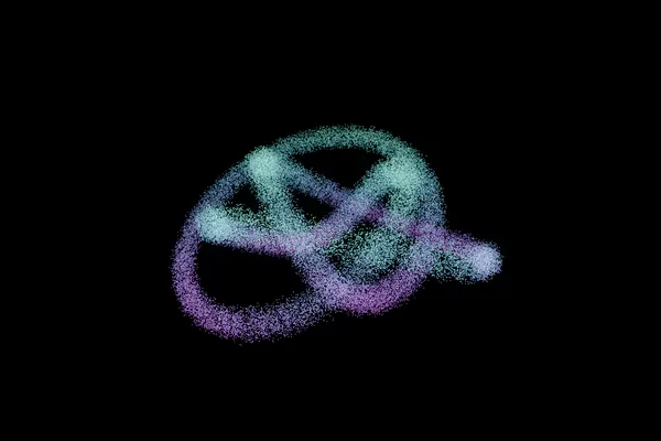
figure-eight knot
gen:figure-eight
the only knot with four crossings, and the simplest one that is its own mirror image
fractals
Self-similar at every scale, found by the chaos game, by escape time, or by marching rays inward until they stop escaping.
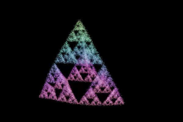
Sierpinski
gen:sierpinski
the Sierpinski tetrahedron, by the chaos game
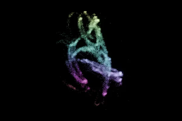
flame
gen:flame
a fractal flame — the chaos game over a few curling maps, each an affine step bent by the paper's variations; which maps a point came through is its depth, so the strands open into layers as it turns
knobs seed which maps and variations; a draw that collapses or hazes over is passed for the next (any whole number, default 4)
Scott Draves & Erik Reckase, “The Fractal Flame Algorithm” (2003)
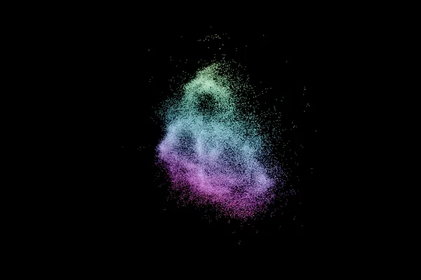
Buddhabrot
gen:buddhabrot
where the Mandelbrot set's escaping points go on their way out — millions of orbits counted, a seated figure in their density; depth is how long each took to escape
knobs low the fewest steps an orbit may take to escape and still count; higher clears the fog (2 to 2000, default 20)
high the most steps an orbit is followed for (50 to 20000, default 2000)
Melinda Green, the Buddhabrot (1993); Lori Gardi’s Nebulabrot
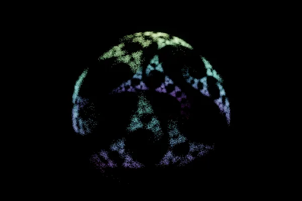
Kleinian
gen:kleinian
a Kleinian limit set — where every orbit of a group of two Möbius maps piles up, a necklace of pearls on the Riemann sphere; both traces at 2 is the Apollonian gasket
knobs ta the trace of a, real part (1.5 to 3, default 1.87)
ta_i the trace of a, imaginary part (-1 to 1, default 0.1)
tb the trace of b, real part (1.5 to 3, default 1.87)
tb_i the trace of b, imaginary part (-1 to 1, default -0.1)
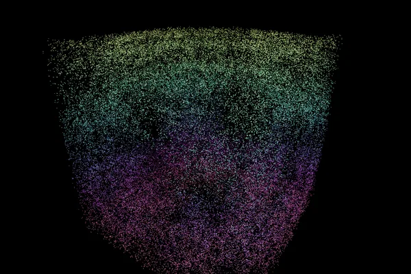
Menger
gen:menger
the Menger sponge, by the chaos game
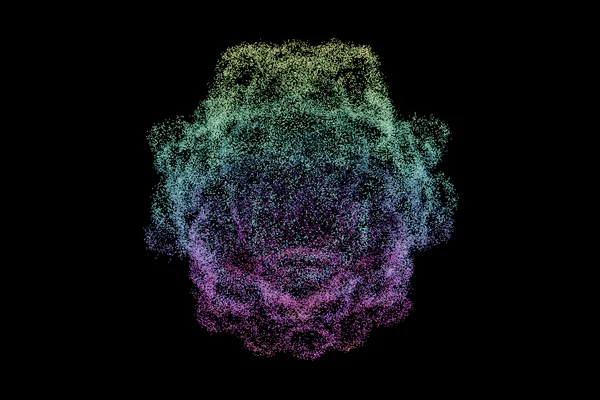
Mandelbulb
gen:mandelbulb
the power-eight Mandelbulb's surface, found by marching rays inward
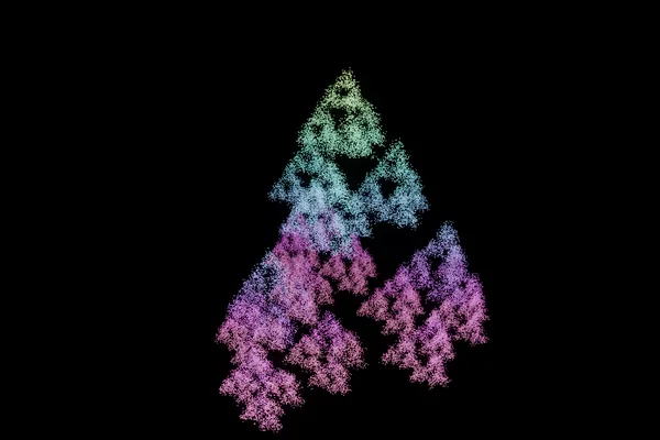
twisted gasket
gen:kifs
the Sierpinski tetrahedron with a turn folded into every step — shells, spirals and lattices, one number wide
knobs angle degrees of turn per step; 0 is the plain gasket (-180 to 180, default 24)
tilt degrees of turn about the other axis (-180 to 180, default 0)
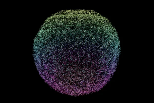
Mandelbox
gen:mandelbox
fold, invert, scale, add — where the Mandelbulb is organic, this is architecture
knobs scale the multiplier in the iteration; negative values turn it inside out (-4 to 4, default 2)
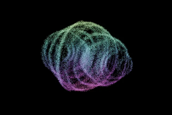
quaternion Julia
gen:quaternion
z ← z² + c in four dimensions, sliced back into three
knobs cr the real part of c (-2 to 2, default -0.2)
ci the first imaginary part (-2 to 2, default 0.6)
cj the second imaginary part (-2 to 2, default 0.2)
Alan Norton, “Generation and display of geometric fractals in 3-D”, SIGGRAPH 1982
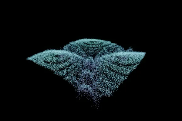
Newton
gen:newton
Newton's method for zⁿ = 1 as a relief — basins whose boundary touches every basin at once
knobs power how many roots to chase (2 to 8, default 3)
Arthur Cayley asked the question in 1879 and could not answer it for the cubic
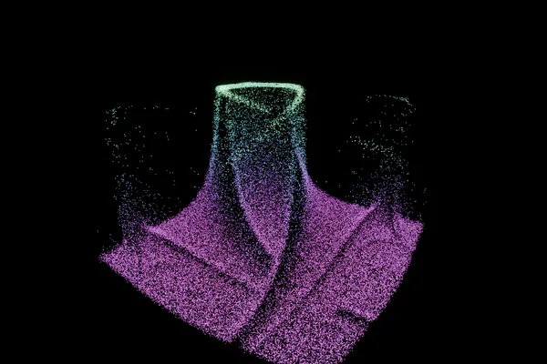
Lyapunov
gen:lyapunov
the Markus–Hess fractal — where the logistic map settles into a cycle, drawn as towers over the chaotic sea
knobs sequence which rate, in turn: AB is the published one, AABAB is another city (text, default AB)
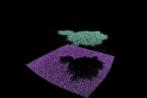
Mandelbrot
gen:mandelbrot
the Mandelbrot set as a relief — the set a plateau, the escape time the country round it
Benoit Mandelbrot (1980); the smooth escape count is Douady and Hubbard’s
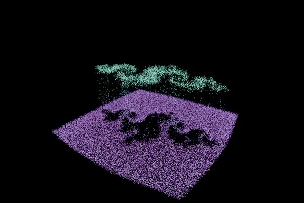
Julia
gen:julia
a Julia set as a relief, c = −0.8 + 0.156i
knobs cr the real part of c (-2 to 2, default -0.8)
ci the imaginary part of c (-2 to 2, default 0.156)
grown
Built step by step by a rule, rather than evaluated: rewriting an alphabet, or letting particles wander in and stick.
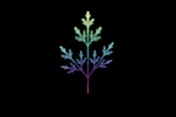
plant
gen:plant
a plant grown by an L-system — five generations of branching, thick wood to thin twigs
knobs rule the production for X — F draws, + − & ^ \ / turn, [ ] branch, X grows again (text, default F[+&X][-^X]/F[\X]X)
angle degrees per turn (5 to 60, default 25)
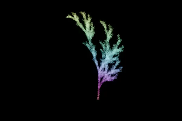
fern
gen:fern
a fern by Lindenmayer's rewriting — fronds off a curling spine, rolling as they go
knobs angle degrees per turn (5 to 60, default 22)
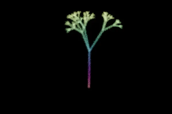
coral
gen:coral
a three-way branching coral — every tip splits into three, a third of a turn apart
knobs angle degrees per turn (5 to 60, default 30)
The same rewriting, branching three ways a third of a turn apart
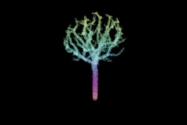
colonised tree
gen:colonise
a tree that finds its own shape — a crown of points pulls on the nearest branch tips, each tip grows towards what pulls it, and a point is used up once a branch reaches it; the trunk thickens by the pipe rule
knobs seed where the crown's points fall (any whole number, default 1)
density how full the crown is: more points, more and finer branches (0.2 to 3, default 1)
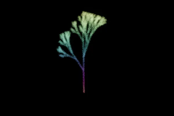
tree
gen:tree
a tree with a trunk — long wood below, short twigs above, branches off three sides
knobs angle degrees per turn (5 to 60, default 20)
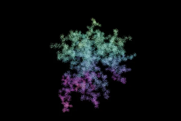
aggregate
gen:dla
diffusion-limited aggregation — particles that wander in and stick where they touch; soot, lightning and copper all do this
knobs seed which walk; the same seed is the same dendrite (any whole number, default 1)
patterns
Sampled where a pattern is, rather than swept: a point is kept if the field says so.
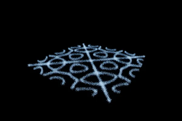
Chladni
gen:chladni
sand on a vibrating plate — points settle where the plate stands still
knobs n the first mode number (1 to 9, default 5)
m the second; equal numbers make no pattern (1 to 9, default 2)
Ernst Chladni, Entdeckungen über die Theorie des Klanges (1787)
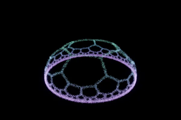
hyperbolic
gen:hyperbolic
a regular tiling of the hyperbolic plane, p-gons q to a corner, as in Escher's Circle Limit prints — the Poincaré disc lifted onto the dome above it, so every edge is a half-circle
knobs p sides to a tile (3 to 12, default 7)
q tiles to a corner; (p − 2)(q − 2) must pass 4 (3 to 12, default 3)
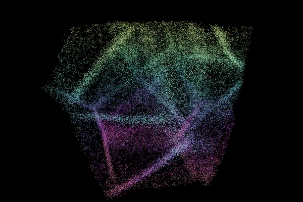
foam
gen:voronoi
Voronoi foam — the walls between cells scattered in a box, meeting three at an edge as soap films do
knobs cells how many centres to scatter (4 to 64, default 24)
seed where they land (any whole number, default 1)
Georgy Voronoy (1908); the walls are the set of points equidistant from the two nearest centres
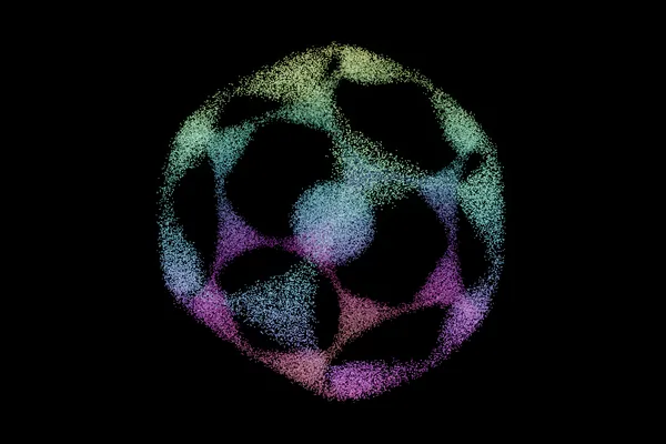
quasicrystal
gen:quasicrystal
six plane waves on the five-fold axes of an icosahedron — a pattern that never repeats and is nowhere random
knobs cells how fine the pattern is (1 to 8, default 3)
Dan Shechtman et al., Phys. Rev. Lett. 53 (1984); Nobel Prize in Chemistry, 2011
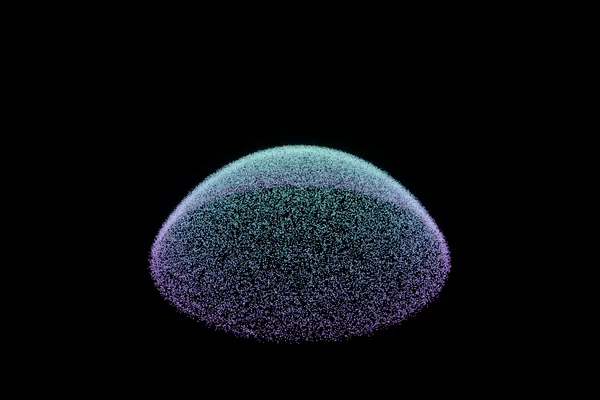
phyllotaxis
gen:phyllotaxis
the sunflower's own packing — one floret every 137.5°, the only angle that never lines up
knobs angle degrees between florets; a tenth off the golden angle and the spiral arms appear (1 to 359, default 137.50776)
rise how far the head domes (0 to 3, default 0.6)
22 that are alive
These are not made once. Each runs on a thread of its own at the frame rate and streams into the live slot, driven by whatever the audio input is doing: the four bands, the loudness, and where the bar is. That is the whole interface they get — deliberately, because the point is a cloud that happens to be alive rather than a second engine with its own controls.
The plates below are each one caught a couple of seconds in, with no audio playing. The ones that are about growing were given longer.
curves
Drawn as one path, in order, so the crawl runs along it and the lines stroke draws it as wire.
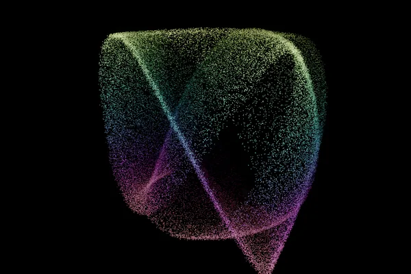
scope
sim:scope
an oscilloscope in XY mode — left across, right up, the last second of the signal trailing back into the screen; a tone is a loop, two tones a Lissajous figure, oscilloscope music a picture; a mono input is drawn against itself a moment earlier
The XY mode of the cathode-ray oscilloscope; Jerobeam Fenderson, “Oscilloscope Music” (2016)
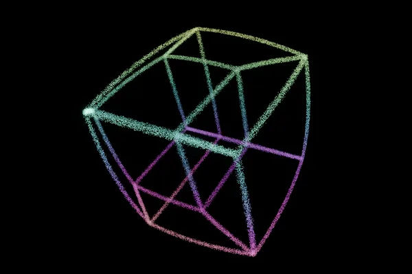
polytope
sim:polytope
a regular solid of four dimensions, turning through the fourth and seen in ours — its cells swell towards you, pass through each other and shrink away, so it turns itself inside out; drawn as one unbroken walk along every edge, so lines draw the wireframe; the loudness turns it and the kick throws it
knobs kind 5-cell, tesseract, 16-cell, 24-cell, 600-cell or 120-cell (text, default tesseract)
grown
Built step by step by a rule, rather than evaluated: rewriting an alphabet, or letting particles wander in and stick.
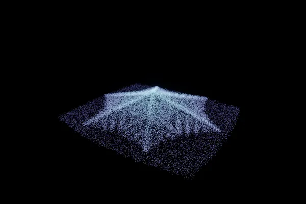
crystal
sim:crystal
Reiter's snow crystal on a hexagonal lattice — plates, sectored plates and stellar dendrites, sorted by the vapour the mids and highs set; each flake grows out and the next one starts
growth
sim:growth
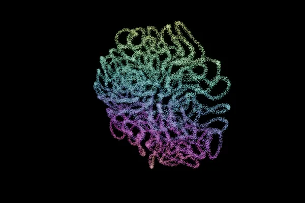
differential growth — one closed thread that grows faster than it has room for and buckles into a coral meander to fit, never crossing itself; the loudness is the growth rate, the kick buds a lobe, and when it is grown it starts again
fields
A grid of numbers stepped forward sixty times a second. The cloud is what rides it.
fluid
sim:fluid
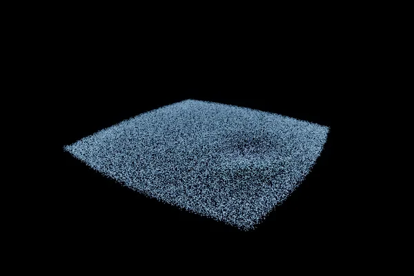
Stam's stable fluids — the Navier–Stokes equations on an endless sheet; the loudness stirs it, the kick bursts it, the snare spins it, the highs roughen it
reaction
sim:reaction
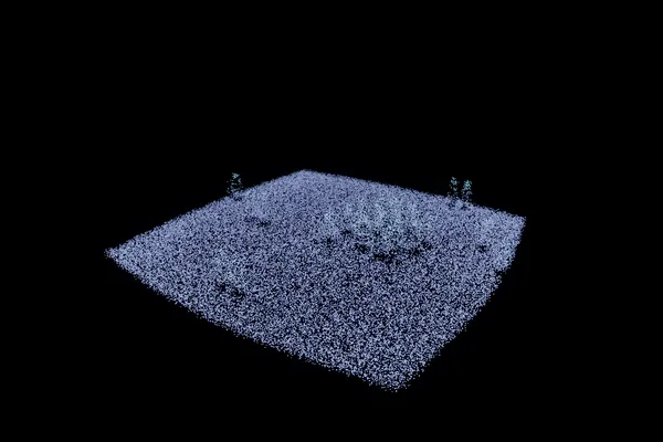
Gray–Scott reaction–diffusion — spots that grow, split and heal; the kick plants new ones
wind
sim:wind
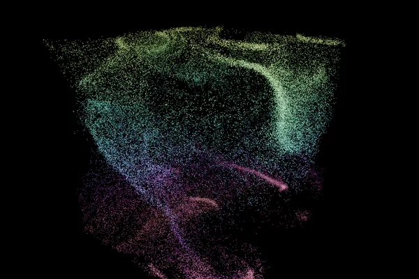
curl noise — tracers in a divergence-free noise field, a fluid with no solve; the kick is a gust, the highs roughen it
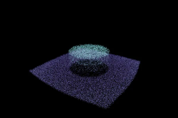
sandpile
sim:sand
grains dropped and toppled — the model that named self-organised criticality, and a fractal nobody designed; the kick drops a load somewhere else
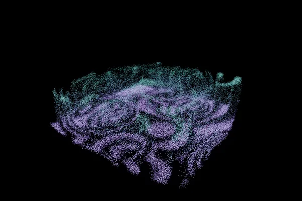
spirals
sim:spiral
the Belousov–Zhabotinsky reaction — rotating waves that annihilate where they meet, the same dynamics as a heartbeat; the kick seeds fresh defects
Boris Belousov (1951) and Anatol Zhabotinsky (1964); the cellular form is Alasdair Turner’s
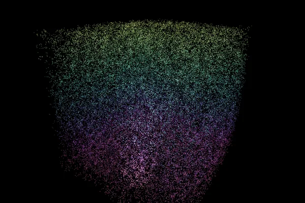
smoke
sim:smoke
the same solver in three dimensions, with heat — a plume that rises, shears and rolls up; the kick is a blast, the snare a shove, the highs the roughness
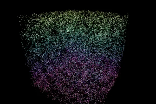
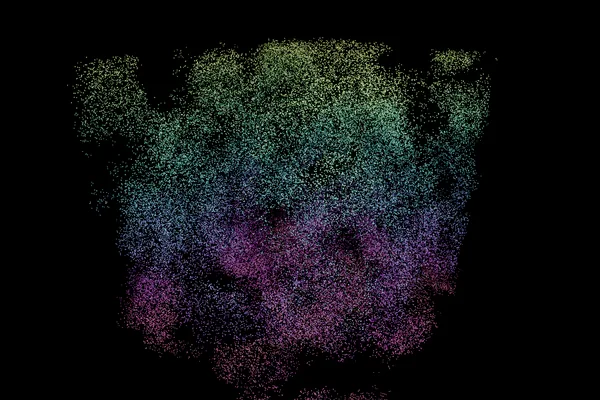
cyclic
sim:cyclic
states in a ring, each waiting to be eaten by the next: noise organises itself into scroll waves that turn for ever, because a spiral's own wave comes back round to feed it
life
sim:life
a three-dimensional cellular automaton in the Pyroclastic rule — a lattice that boils, endlessly; the kick drops a seed
knobs rule survive / born / states, as neighbour counts: 4-7/6-8/10 is Pyroclastic and boils; 2,6,9/4,6,8-9/10 builds; 4/4/5 is Bays' 4-4-5, a spiking crystal; 13-26/13-14,17-19 is Clouds, which grows lovely masses and then stops, so it is started again (text, default 4-7/6-8/10)
many bodies
Many things, each with a position of its own, and rules about how they see each other.
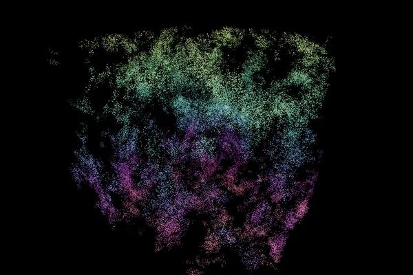
flock
sim:flock
Reynolds' boids — four thousand of them drawing streaks; the loudness is their pace, the kick a predator, the snare a scatter
Craig Reynolds, “Flocks, Herds and Schools: A Distributed Behavioral Model”, SIGGRAPH 1987
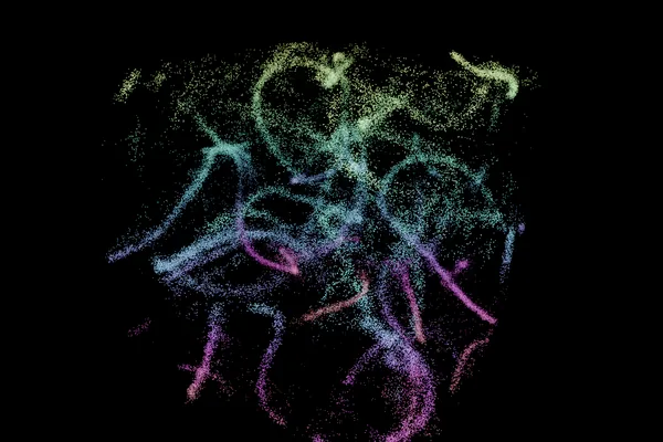
slime
sim:slime
Physarum: sixty-five thousand agents that leave a trail and follow the strongest one they can see — a transport network out of three rules and no plan; the kick starts a new front
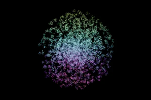
swarmalators
sim:swarm
particles that swarm and synchronise at once, each depending on the other — five states from two numbers; the loudness and the mids move between them
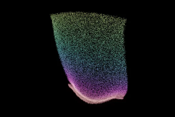
cloth
sim:cloth
a sheet of sixty-five thousand particles hung from its top edge in an Arnold–Beltrami–Childress wind; the kick is a gust
Xavier Provot, “Deformation constraints in a mass-spring model”, Graphics Interface 1995; Thomas Jakobsen, “Advanced Character Physics”, GDC 2001
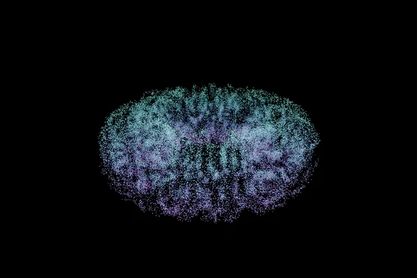
kuramoto
sim:kuramoto
Kuramoto's coupled oscillators on a torus — a loud passage locks them into a ribbon, quiet frees them; the kick scatters half
Yoshiki Kuramoto (1975); Steven Strogatz, “From Kuramoto to Crawford”, Physica D 143 (2000)
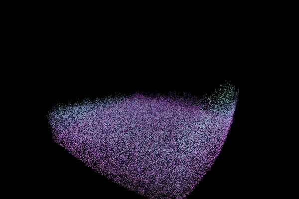
liquid
sim:liquid
four thousand particles of water in a tilting box — gravity swings round once a bar, so it pours corner to corner; the kick throws it at the ceiling
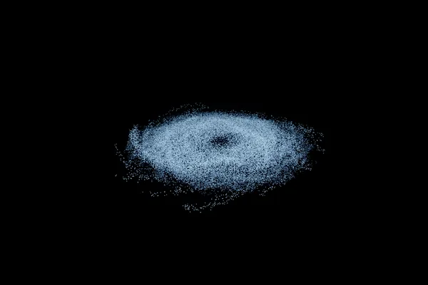
orbits
sim:orbits
five hundred bodies pulling on each other round a heavy centre — the loudness is the clock, the kick a shockwave, the snare knocks the disc out of its plane
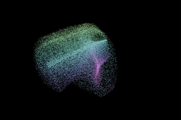
pendulum
sim:pendulum
four thousand double pendulums hung in a sheet from neighbouring angles — it swings as one surface, creases, then tears; the loudness is gravity and the kick hangs it again
The double pendulum, the standard demonstration that four numbers can be unpredictable
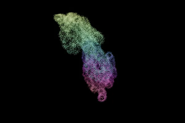
tangle
sim:tangle
one long elastic rod loose in a wind, tying itself in knots — it cannot stretch and it cannot pass through itself, which is the difference between a tangle and a scribble
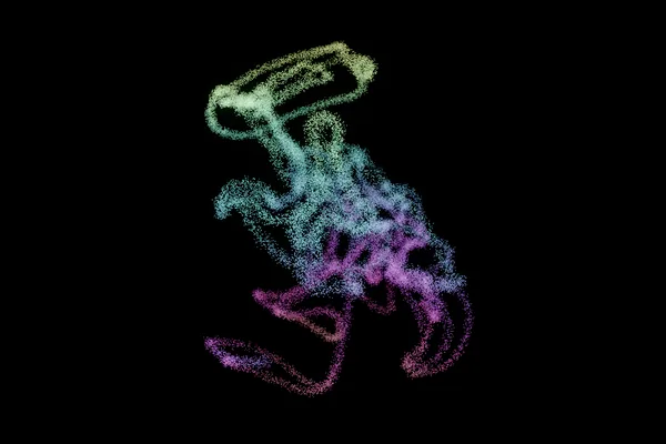
vortex
sim:vortex
the thin cores smoke rings are made of, moving each other by Biot–Savart — rings that catch the one in front and thread through it; the loudness is their circulation and the kick throws a new one in
The rest of the picture
The clouds are the part of vizz with the longest bibliography, but they are not the only part of it that came from somewhere. What follows is the same treatment for everything else a frame is made of — the shapes the shader draws without a slot, the pattern stack, the colour, the light, the listening and the passes at the end.
A source here is the idea, not the implementation: all of it is written out in this repository rather than pulled in as a library, so where a paper and the code disagree the entry says how. Where there is nothing outside vizz to cite, the line says so (dashed) rather than leaving a blank that reads like a missing citation.
shapes
A filled slot is not the only way vizz gets a form on screen. These are what /shape/mode sweeps through, and most of them never touch memory at all: the particle's index is hashed into four numbers and the shape is a function of those four, evaluated in the vertex stage. That is why the sweep can morph one into the next — a particle keeps its hashes, so the same point travels between forms rather than the field being scattered again.
Solid sphere and hollow shell
Both are sampled uniformly by volume rather than by angle, which is the difference between a sphere and a sphere with a bright clot at each pole. Height is drawn uniformly from −1 to 1 and the ring radius follows from it; for the solid sphere the radius is scaled by the cube root of a uniform draw, and for the shell it stays near the surface.
Source: the uniform-height trick is Archimedes' hat-box theorem — equal slices of a sphere carry equal area — in the form usually written up as sphere point picking.
Trefoil knot
The simplest non-trivial knot, drawn as a core curve and thickened into a tube by scattering particles around it. vizz uses the standard (2, 3) torus-knot parametrisation. The catalogue above has a knot of its own with p and q to turn; this one is fixed, because it is a stop on a sweep rather than a cloud you configure.
Source: classical knot theory; the parametrisation is the standard one, as given on MathWorld.
Lorenz and Aizawa
The two attractors that predate the catalogue. Unlike the rest of the sweep these are not evaluated per vertex: both are integrated once on the CPU at startup — Lorenz with σ 10, ρ 28, β 8/3, the classic values — the first 20,000 steps discarded as transient, and the next 65,536 stored in trajectory order in the first two cloud slots. Consecutive points are consecutive moments, so advancing every particle's index makes the cloud crawl along the attractor rather than shimmer in place. Aizawa is there as a contrast partner: rounder, shell-like, with a spike through the poles, so the morph between the two has somewhere to go. Both appear in the catalogue above as well, where they can be asked for by name into any slot.
Source: Edward N. Lorenz, “Deterministic Nonperiodic Flow”, Journal of the Atmospheric Sciences 20(2), 1963. Aizawa is named for Yoji Aizawa, whose work on chaotic flows it comes out of; unlike Lorenz it has no single canonical paper behind it, and the parameter set vizz uses is the one that circulates in graphics, stated the same way in Analog Paradigm's write-up.
Torus, grid plane, cloud pair
A torus from its two angles, a grid plane with a travelling ripple, and the cloud pair — which is not a shape at all but a blend between any two loaded slots: a scan, an attractor, a word, a live video frame. The sweep only reaches adjacent modes, so crossing a scan into an attractor needs a control of its own, which is what /cloud/morph is.
Source: plain parametric forms with nothing behind them worth citing.
Wind
A displacement laid over whatever shape is showing, so a still form leans and breathes without becoming a simulation. Two octaves of one field, each drifting at its own pace so the wind never settles into a pattern the eye can lock onto. It runs per vertex, on every form including a loaded scan, because the field it uses is six trigonometric terms — a curl of noise would not fit there.
Source: the Arnold–Beltrami–Childress flow with A = B = C = 1: a steady solution of the Euler equations, divergence-free by construction, and chaotic in its streamlines — the standard example of a simple field that mixes.
layers
The print-look counterpart to the particle field, and the other half of what vizz puts on a screen.
The stack
Eight procedural pattern layers — rings, stripes, checker, polygon, star, rays, dots — in flat ink colours on coloured paper, each with its own similarity transform, drawn in a single fullscreen pass and composited in-register.
Source: 555-5555's visuals for Caribou's live shows, which is the look this was built to reach. Not an algorithm and not a paper — an idiom, borrowed knowingly. The generators themselves are ordinary procedural patterns.
Moiré
The reason the stack has eight layers and not one. Two periodic patterns at close frequencies interfere into a third, much coarser pattern that neither layer contains, and it moves far faster than either layer does when you drift one of them. The built-in show is largely made of this.
Source: Isaac Amidror, The Theory of the Moiré Phenomenon, Volume I: Periodic Layers, Springer.
Blend modes
Multiply, screen, add, difference, exclusion and subtract, the vocabulary the look is built in.
Source: the separable blend modes of W3C Compositing and Blending Level 1. vizz departs from the spec in one deliberate way: it blends on sRGB-encoded values rather than linear ones, because compositing on encoded values is the print-era behaviour this aesthetic grew out of. The single conversion to linear happens on the way out of the shader.
Analytic antialiasing
Hard-edged patterns alias badly, and the usual fix — fwidth — lies at exactly the discontinuities these patterns are made of. Instead each layer carries one scalar for how many pattern units a pixel spans, propagated by the chain rule through the layer transform, and each generator turns a signed distance into coverage over that footprint. Past Nyquist the coverage converges to flat duty-cycle tone, so the moiré survives where the sparkle does not.
Source: the technique Iñigo Quilez describes in “filtering procedural textures”. The per-generator gradient magnitudes are worked out for these generators specifically.
colour
What comes out of the shader, and what stops it turning to white.
Cosine palettes
The four built-in gradients are colour = a + b·cos(τ(c·t + d)), four coefficients each. They are baked into a lookup texture on the CPU rather than evaluated in the shader, so a palette you load from a list of colour stops sits in the same bank and is indistinguishable from a built-in as far as the renderer is concerned.
Source: Iñigo Quilez, “palettes”.
HSV
Palette 0 stays procedural rather than baked, so /particles/hue keeps meaning a rotation through hue rather than an offset into a ramp.
Source: Alvy Ray Smith, “Color Gamut Transform Pairs”, SIGGRAPH 1978 — the paper HSV comes from.
The tone shoulder
Glow and trails push values well past 1, and a hard clip turns highlights into flat white blobs. The composite pass ends with c / (1 + 0.15c), which rolls the top off and leaves midtones essentially untouched. It is the default finish; the graded one below replaces it when asked.
Source: the c/(1+c) curve from Reinhard, Stark, Shirley and Ferwerda, “Photographic Tone Reproduction for Digital Images”, SIGGRAPH 2002. The 0.15 is tuned for this picture, not from the paper.
sRGB
The transfer function the vector stack encodes and decodes with, and the one the output textures are in.
Source: IEC 61966-2-1.
light
A cloud of dots has no surface, which makes lighting one a question rather than a setting.
Estimated normals
Most scanners export points with no surface direction, and the sun cannot light a surface it cannot orient. vizz reads normals from a PLY that carries them and works them out from each point's twelve nearest neighbours when it does not: fit a plane through the neighbourhood, and the plane's normal is the surface's — the eigenvector of the neighbourhood's covariance with the smallest eigenvalue.
Source: Hoppe, DeRose, Duchamp, McDonald and Stuetzle, “Surface Reconstruction from Unorganized Points”, SIGGRAPH 1992, where the local plane fit is step one. vizz stops there: the paper goes on to propagate a consistent orientation across the cloud, and vizz instead flips each normal towards the eye, which is a better answer for a scan of a room seen from inside it.
Lamps and the sun
Two movable lamps that fall off with distance and work on anything with a position, and a directional sun that lights surfaces — the wall facing it comes up, the wall facing away goes down. A cloud with no normals is left alone by the sun rather than lit from a direction nobody measured.
Source: Lambert's cosine law (Johann Heinrich Lambert, Photometria, 1760) for the directional term. The distance falloff is a smooth r²/(d²+r²) rather than inverse-square, so there is no singularity to divide by on stage.
PLY
The format a scan arrives in, ASCII or binary little-endian, and also the wire format for live point-cloud streaming — there is no wrapper protocol, because a PLY header already states its own frame length. The simulations above reach the renderer down the same pipe.
Source: the Stanford polygon format, Greg Turk, Stanford University.
Depth of field
Done by resizing the sprite rather than blurring the frame: a defocused point light is a larger, dimmer disc, so the particle's billboard grows with its distance from the focus plane and dims by the square of that growth. Closer to the real thing than a post-process blur, and it costs nothing.
Source: vizz, on the ordinary optics of the circle of confusion.
randomness
Where every particle that is not read out of a slot comes from.
The particle hash
Every particle is derived from its index and nothing else — no state carried between frames, which is what makes the count free to change mid-set and the whole field scrubbable. Four independent random streams per particle come out of one integer mixer. It replaced a float hash whose repeats at high counts stacked particles on each other and pushed them into the tone-map shoulder; an integer mixer has no such cliff, and is stable across GPUs in a way anything built on sin() is not.
Source: the lowbias32 constants from Chris Wellons' hash prospector, described in “Prospecting for Hash Functions”.
audio
The four bands, the loudness and the bar — the whole of what the simulations above are driven by, and most of what the rest of the app listens to.
Window and spectrum
A 2048-point FFT at 48 kHz — a 43 ms window, 23 Hz a bin — through a periodic Hann window, with the band magnitudes corrected for the window's power loss so that a band meter and a gain control mean something absolute rather than something relative to the window.
Source: the transform itself is the rustfft crate; the window and its correction factor are from Fredric J. Harris, “On the Use of Windows for Harmonic Analysis with the Discrete Fourier Transform”, Proceedings of the IEEE 66(1), 1978, and Parseval's theorem for the normalisation.
Onset detection
Positive spectral flux: how much energy appeared since the last frame, summing only the bins that went up. Summing the drops as well would make a note ending look like a note starting.
Source: the half-wave-rectified spectral flux detector, surveyed and compared in Simon Dixon, “Onset Detection Revisited”, DAFx-06.
Tempo
Autocorrelation of the onset signal: if the music has a pulse, the onset signal correlates with itself at the beat period, and peak-picking the correlation gives a BPM without anything ever having to decide what a beat is. The characteristic failure is the octave error — 180 for a 90 BPM track — because a signal that correlates at one period also correlates at its multiples. Two guards: a prior preferring the middle of the range, and a check for whether half the candidate explains the signal comparably well. A confidence figure comes out alongside, so ambient material with no pulse reports low confidence rather than a confident wrong answer.
Source: autocorrelation of an onset-strength envelope, as set out in Daniel P. W. Ellis, “Beat Tracking by Dynamic Programming”, Journal of New Music Research 36(1), 2007. vizz uses the tempo-estimation half and not the dynamic-programming beat tracker — a VJ needs the rate, and the phase comes from the pads.
frame
Everything that happens to the picture after the clouds are in it.
Feedback trails
The pass that makes the output look like VJ material. Last frame's result is zoomed and rotated a little and mixed back in with the new one, so motion smears into trails and a sustained zoom builds a tunnel out of whatever is on screen. A lerp rather than an accumulation, because adding the history outright is a geometric series that saturates to white within a second.
Source: analogue video feedback, which is where this whole idiom comes from — Steina and Woody Vasulka's work and the Sandin Image Processor (Dan Sandin, 1971–73). The implementation is an ordinary ping-pong of two Rgba16Float textures.
Kaleidoscope and lens
Mirror, quad mirror and a six-wedge kaleidoscope, all done as a fold of UV space before sampling; a radial RGB split that leaves green alone, so the frame fringes towards the edges the way a lens does instead of shifting hue; and a cheap six-tap bloom.
Source: vizz. Standard screen-space constructions with no particular paper behind them.
Drawing at twice the size
Up to 1080p the frame is drawn at twice the output's width and height and filtered down, which is the one thing that reliably cleans up a field of one-pixel sprites: against a 4× reference it takes out about half the error and more than half the frame-to-frame shimmer. Two things had to change for that to be safe. The room's lines were one-pixel hardware lines, so drawn at 2× they lost half their light; they are now quads one output pixel wide whose edge coverage is the exact overlap of a pixel with the line, so the room is equally bright at any scale and anti-aliased at 1× as well. And a sprite smaller than about a pixel and a half is widened to that size and dimmed by the area it gained, so it is low-passed instead of landing on a pixel centre or missing it.
Source: the line coverage is the box-filter case of Satish Gupta and Robert Sproull, “Filtering Edges for Gray-Scale Displays”, SIGGRAPH 1981. The sprite floor is the screen-space filter of Zehao Yu, Anpei Chen, Binbin Huang, Torsten Sattler and Andreas Geiger, “Mip-Splatting: Alias-free 3D Gaussian Splatting”, CVPR 2024, applied to a disc instead of a Gaussian.
The graded finish
An alternative to the shoulder, faded in with /fx/grade. Three things change together. The exposure is metered: a histogram of log luminance over the lit pixels every frame, with the exposure eased towards putting the brightest one percent on the curve's shoulder. In the app the meter only ever darkens, so a look that clips is pulled back while a fade still reaches black. The glow becomes a mip chain: the frame halved six times and summed back up, so it falls off from a sharp core to a wide haze instead of showing its taps. And the curve is AgX, which compresses highlights over about sixteen stops in log space and desaturates as it goes, so a dense core of coloured sprites reads as a hot centre fading into its colour rather than a flat disc of clipped primary. The background is taken out before grading and put back after, so a colour chosen to match a room stays that colour. Every plate on this page is drawn through it, metered per plate.
Source: the curve is Troy Sobotka's AgX, in the polynomial fit from Benjamin Wrensch's “Minimal AgX Implementation” (2023). The bloom filters are from Jorge Jimenez, “Next Generation Post Processing in Call of Duty: Advanced Warfare”, SIGGRAPH 2014: a thirteen-tap downsample, Karis-averaged on the first step, and a tent on the way up. Metering from a percentile of a log-luminance histogram is how game engines' auto-exposure works, Unreal's among them.
Gaussian splats
/particles/splat draws every particle as a soft, oriented ellipse of colour, blended over the frame from the farthest to the nearest, so the near ones cover the far ones instead of adding up to light. A cloud loaded from a 3D Gaussian Splatting capture keeps each splat's own size, turn, opacity and colour, so the capture renders as the photographs it was trained from and still turns and morphs like any cloud; anything else is drawn as round splats of the particle size. Each frame a compute pass evaluates every particle with the dots' own functions and carries its ellipsoid to the screen through the projection's Jacobian, a bitonic sort orders them by depth, and a draw lays a quad over each with premultiplied “over” blending. Only the colour's first spherical-harmonic band is read, so a capture's colours do not shift with the view.
Source: Bernhard Kerbl, Georgios Kopanas, Thomas Leimkühler and George Drettakis, “3D Gaussian Splatting for Real-Time Radiance Field Rendering”, SIGGRAPH 2023, for the format and the method; the projection is the EWA splatting of Matthias Zwicker, Hanspeter Pfister, Jeroen van Baar and Markus Gross, “EWA Volume Splatting”, IEEE Visualization 2001; the sort is Kenneth Batcher's bitonic network, “Sorting networks and their applications”, AFIPS 1968.
Haze and light beams
/light/haze fills the space in front of the camera with a lit medium, like stage haze, and /light/smoke lets the particles thicken it, so a cloud becomes smoke that the lamps and the sun cut through. The space is cut into froxels, a grid that is a coarse pixel grid across and slices of distance deep; each frame every particle is shared among the eight froxels round it, each froxel is lit by both lamps and the sun with each light dimmed by the smoke between them, and the light is gathered front to back along each column. Light coming through the gaps in a lattice, a tree or an open attractor makes beams, and the smoke's own shadow makes shafts. /light/scatter is the Henyey-Greenstein anisotropy, how much brighter the haze is looking towards a lamp than across it.
Source: Bartłomiej Wroński, “Volumetric Fog and Lighting”, SIGGRAPH 2014 Advances in Real-Time Rendering, for the froxel volume; Sébastien Hillaire, “Physically Based and Unified Volumetric Rendering in Frostbite”, SIGGRAPH 2015, for the integration; single scattering as Nelson Max sets it out in “Optical Models for Direct Volume Rendering”, IEEE TVCG 1995; the phase function of Louis Henyey and Jesse Greenstein, “Diffuse radiation in the galaxy”, Astrophysical Journal 1941.
Solid surfaces
With /particles/surface up, a particle stops being light and becomes a small opaque disc, so the cloud is an object: nearer discs hide farther ones, a lamp lights the side of the form that faces it, and the sun casts a shadow onto the cloud itself and onto the room, which is drawn as walls, floor and ceiling instead of lines. Each particle is evaluated once by a compute pass with the same functions the glowing mode uses, so switching never moves anything. The lighting is deferred: the discs write colour and depth, and one pass lights every pixel, reading which way the surface faces from the depth a few discs away on each side. That is what lets a procedural sphere with no normals at all shade as a sphere rather than a heap of beads.
Source: the discs are surfels, after Hanspeter Pfister, Matthias Zwicker, Jeroen van Baar and Markus Gross, “Surfels: Surface Elements as Rendering Primitives”, SIGGRAPH 2000. The shadow is a shadow map, Lance Williams, “Casting Curved Shadows on Curved Surfaces”, SIGGRAPH 1978, read with the percentage-closer filtering of William Reeves, David Salesin and Robert Cook, “Rendering Antialiased Shadows with Depth Maps”, SIGGRAPH 1987. Normals from the depth buffer are standard deferred-rendering practice; the span that follows the surfel size is vizz's.
Lines and streaks
With /particles/stroke a glowing particle can be drawn as more than a dot. A line draws each particle back along its own path at the present moment: a cloud keeps its trajectory in time order, so on a flow or a curve thousands of short strokes join up into the path itself, and the Lorenz butterfly becomes wire instead of dust. A streak draws each particle back through time instead, fading towards where it was, which is motion blur, and it shortens to a dot when nothing moves. Both are ribbons of four segments turned to face the eye, spending four quads of the particle budget, so the cost of a frame does not change; and each carries its particle's light spread along it, so a long stroke is fainter rather than brighter.
Source: lines after Malte Zöckler, Detlev Stalling and Hans-Christian Hege, “Interactive Visualization of 3D-Vector Fields Using Illuminated Stream Lines”, IEEE Visualization 1996. Streaks after William Reeves, “Particle Systems — a Technique for Modeling a Class of Fuzzy Objects”, SIGGRAPH 1983, which drew each particle as a motion-blurred streak.
Plexus
/particles/plexus draws lines between the particles that come near each other: the network, or the constellation, over any cloud and in either draw mode. Up to 2048 of the particles, spread evenly over the whole field, are the nodes. Each frame a compute pass places them with the dots' own shader functions, and a second finds each one's four nearest within /particles/plexus_reach by testing every other node — a few million distance tests, which needs no grid. A thin additive line runs along each link in the colours of its two ends, fading to nothing as the pair drifts out of reach, so links come and go softly instead of snapping. A pair that lists each other is drawn once.
Source: the motion-graphics “plexus” look, after Rowbyte's Plexus plug-in for After Effects (2010), whose name it has become; the geometry is a k-nearest-neighbour graph cut at a radius.
Glyphs
In the surface mode, /particles/glyph makes each particle a small solid instead of a disc: a tetrahedron, a cube, an octahedron, a long shard or a mix. Each is turned to the way its particle travels, found by evaluating the particle a twentieth of a second of visual time earlier, rolls slowly about that axis, and is lit by its own exact face normals, so the facets catch the light as facets. The glyphs cast their own shapes into the shadow map. A disc says the cloud is a surface sampled by points; a glyph says it is a field of things.
Source: Rita Borgo, Johannes Kehrer, David H. S. Chung, Eamonn Maguire, Robert S. Laramee, Helwig Hauser, Matthew Ward and Min Chen, “Glyph-based Visualization: Foundations, Design Guidelines, Techniques and Applications”, Eurographics State of the Art Reports, 2013.
Fractal solids
In the surface mode, /particles/solid draws a fractal as a lit, opaque solid where the cloud sits: the Mandelbulb, the Mandelbox, a quaternion Julia set or the Menger sponge. None of them is made of particles. Each pixel marches a ray from the camera, stepping each time by the fractal's distance estimate — a bound on how far the nearest surface can be — until it is within a pixel of the surface, and writes its colour, its exact normal and its depth into the same buffers the cloud fills, so the two hide each other properly and are lit by the same lamps. A ray that needed many steps to get in found a crevice, and is darkened for it. /particles/solid_detail is the one knob: the bulb's power, the box's scale, the turn of the Julia constant, the sponge's depth.
Source: sphere tracing is John C. Hart, “Sphere tracing: a geometric method for the antialiased ray tracing of implicit surfaces”, The Visual Computer 12, 1996; the quaternion Julia estimate is Hart, Sandin and Kauffman, “Ray tracing deterministic 3-D fractals”, SIGGRAPH 1989. The Mandelbulb is Daniel White and Paul Nylander's, 2009; the Mandelbox is Tom Lowe's, 2010; the sponge is Karl Menger's, 1926, with the distance function and the tetrahedral normal from Íñigo Quílez.
Ink
In the surface mode, /particles/ink draws the lit surface as a pen drawing. Outlines go where the depth breaks: at a silhouette, at a fold or an overlap where the depth's second difference jumps, and, on surfaces whose normals are exact (glyphs, solids, walls), where the normal turns. Hatching then lays the tone down on paper as up to three layers of crossed lines, each coming in where the surface took less light than the last; stipple lays it down as dots on a jittered grid, more and larger in the dark. The tone is the light that fell on the surface as a share of all the light in the rig, not the brightness of its colour, so a dark palette is not drawn as a dark form. The marks are fixed to the screen and the outlines move with the form. /particles/ink_weight is how heavy the pen is.
Source: edges from the depth buffer are Takafumi Saito and Tokiichiro Takahashi, “Comprehensible Rendering of 3-D Shapes”, SIGGRAPH 1990; hatching by tone after Emil Praun, Hugues Hoppe, Matthew Webb and Adam Finkelstein, “Real-Time Hatching”, SIGGRAPH 2001, reduced to three screen-space layers; stipple after Adrian Secord, “Weighted Voronoi Stippling”, NPAR 2002, on a jittered grid without the relaxation.
Liquid
In the surface mode, /particles/liquid melts the discs into one glossy surface. After the discs are drawn, one pass blurs the depth they left, as a distance along each pixel's ray, over a few discs' width on screen; the blur is bilateral, so a disc much nearer or farther than the centre counts for little and the surface does not run across a gap into whatever is behind it. The lighting then reads its normals from the smoothed depth, so the bumps of the separate discs are gone, and shades it as a liquid: the light that gets in, tinted by its colour, and on top the sky and sharp highlights of the lamps and the sun, more of them at a glancing angle. Glyphs, solids and the walls keep their own exact surfaces.
Source: screen-space fluid rendering, after Wladimir J. van der Laan, Simon Green and Miguel Sainz, “Screen Space Fluid Rendering with Curvature Flow”, I3D 2009, with a bilateral blur in place of the curvature flow; the Fresnel term is Christophe Schlick, “An Inexpensive BRDF Model for Physically-based Rendering”, Computer Graphics Forum 13(3), 1994.
Gravity wells
Four attractors and repulsors bending the cloud from a layer above the scenes. Deliberately not a simulation: every particle here is a function of its index with no state between frames, and integrating velocities would throw that away for physics nobody is checking. The falloff is r²/(d²+r²) — one at the centre, a half at the radius, asymptotically nothing beyond — because a hard cutoff shows up as a visible shell in the cloud.
Source: vizz. A displacement field that reads as gravity, not a gravity model.
Camera moves
Ten paths — orbit, sway, push, pull, crane, spiral, look around, fly through, walkthrough and a slow drift — each returning a delta added to the camera the faders already describe, with rate in bars so a move locks to the same clock as the sequencer.
Source: vizz. The shapes are borrowed from camera work rather than from anything written down.
Sources
Every entry above, in one list, with whoever found it. Where the original paper is behind a paywall the link goes to an encyclopaedia article instead — the citation is the thing to keep.
The clouds
- aggregate — Thomas Witten & Leonard Sander, “Diffusion-limited aggregation, a kinetic critical phenomenon”, Phys. Rev. Lett. 47 (1981)
- Aizawa — Yoji Aizawa & Tatsuo Uezu (1982), as catalogued by Chaoscope
- Arneodo — Alain Arnéodo, Pierre Coullet & Charles Tresser (1981)
- Boy's surface — Werner Boy (1901); this parametrisation is François Apéry’s (1986)
- Buddhabrot — Melinda Green, the Buddhabrot (1993); Lori Gardi’s Nebulabrot
- Burke–Shaw — Bill Burke & Robert Shaw (1981)
- Chen — Guanrong Chen & Tetsushi Ueta, “Yet another chaotic attractor”, Int. J. Bifurcation and Chaos 9 (1999)
- Chladni — Ernst Chladni, Entdeckungen über die Theorie des Klanges (1787)
- Chua — Leon Chua (1983); Matsumoto, Chua & Komuro, IEEE Trans. Circuits and Systems 32 (1985)
- Clifford — Clifford Pickover, Computers, Pattern, Chaos and Beauty (1990)
- cloth — Xavier Provot, “Deformation constraints in a mass-spring model”, Graphics Interface 1995; Thomas Jakobsen, “Advanced Character Physics”, GDC 2001
- colonised tree — Adam Runions, Brendan Lane & Przemysław Prusinkiewicz, “Modeling Trees with a Space Colonization Algorithm” (2007)
- coral — The same rewriting, branching three ways a third of a turn apart
- Coullet — Pierre Coullet, Charles Tresser & Alain Arnéodo (1979) — a jerk system
- crystal — Clifford A. Reiter, “A local cellular model for snow crystal growth”, Chaos, Solitons & Fractals 23 (2005); the morphologies are Ukichiro Nakaya’s (1954)
- cyclic — Robert Fisch, Janko Gravner & David Griffeath, “Cyclic cellular automata in two dimensions” (1991); David Griffeath on the spirals’ four snapshots (1994)
- Dadras — Sara Dadras & Hamid Reza Momeni, Physics Letters A 373 (2009)
- de Jong — Peter de Jong, in A. K. Dewdney’s Computer Recreations, Scientific American (1987)
- Dini — Ulisse Dini (1870); a pseudosphere dragged along a helix
- Duffing — Georg Duffing (1918); the chaotic forced case is Ueda’s (1979)
- Enneper — Alfred Enneper (1864)
- fern — The same rewriting, in the fern’s own rule
- figure-eight knot — The 4₁ knot, the simplest amphichiral one
- finance — Junhai Ma & Yushu Chen, Applied Mathematics and Mechanics 22 (2001)
- flame — Scott Draves & Erik Reckase, “The Fractal Flame Algorithm” (2003)
- flock — Craig Reynolds, “Flocks, Herds and Schools: A Distributed Behavioral Model”, SIGGRAPH 1987
- fluid — Jos Stam, “Stable Fluids”, SIGGRAPH 1999, and “Real-Time Fluid Dynamics for Games”, GDC 2003; vorticity confinement from Fedkiw, Stam & Jensen, SIGGRAPH 2001
- foam — Georgy Voronoy (1908); the walls are the set of points equidistant from the two nearest centres
- Four-wing — Wang, Sun & van Wyk, the four-wing system (2009)
- Genesio–Tesi — Roberto Genesio & Alberto Tesi, Automatica 28 (1992)
- growth — Anders Hoff, “Differential Line” (inconvergent, 2016); Andy Lomas, “Cellular Forms” (2014); Nervous System’s Floraform (2014)
- Gumowski–Mira — Igor Gumowski & Christian Mira, CERN (1980)
- gyroid — Alan Schoen, Infinite Periodic Minimal Surfaces Without Self-Intersections, NASA TN D-5541 (1970); Schwarz’ P and D are from 1865
- Hadley — Edward Lorenz, “Irregularity: a fundamental property of the atmosphere”, Tellus 36A (1984)
- Halvorsen — Arne Dehli Halvorsen’s cyclically symmetric system, as catalogued by Sprott
- harmonic — A sphere modulated by a spherical harmonic; the classical functions of Laplace (1782)
- Hilbert curve — David Hilbert, “Über die stetige Abbildung einer Linie auf ein Flächenstück”, Math. Annalen 38 (1891)
- Hopf — Heinz Hopf, “Über die Abbildungen der dreidimensionalen Sphäre auf die Kugelfläche”, Math. Annalen 104 (1931)
- hyperbolic — H. S. M. Coxeter, “Crystal symmetry and its generalizations” (1957), after which Escher drew Circle Limit I; Douglas Dunham, “Hyperbolic symmetry” (1986)
- Hénon — Michel Hénon, “A two-dimensional mapping with a strange attractor”, Comm. Math. Phys. 50 (1976)
- Ikeda — Kensuke Ikeda, Optics Communications 30 (1979)
- Julia — Gaston Julia (1918) and Pierre Fatou
- Klein bottle — Felix Klein (1882); the figure-eight immersion is the standard one
- Kleinian — David Mumford, Caroline Series & David Wright, “Indra’s Pearls: The Vision of Felix Klein” (2002), Grandma’s recipe
- kuramoto — Yoshiki Kuramoto (1975); Steven Strogatz, “From Kuramoto to Crawford”, Physica D 143 (2000)
- life — Carter Bays, “Candidates for the Game of Life in Three Dimensions”, Complex Systems 1 (1987); the multi-state rules as catalogued by Softology
- liquid — Miles Macklin & Matthias Müller, “Position Based Fluids”, SIGGRAPH 2013; kernels from Müller, Charypar & Gross, SCA 2003
- Lissajous — Jules Antoine Lissajous (1857); the knotted case is Bogle, Hearst, Jones & Stoilov (1994)
- Lorenz-96 — Edward Lorenz, “Predictability: a problem partly solved”, ECMWF Seminar on Predictability (1996)
- Lyapunov — Mario Markus & Benno Hess, “Lyapunov exponents of the logistic map with periodic forcing”, Computers & Graphics 13 (1989)
- Mandelbox — Tom Lowe (2010)
- Mandelbrot — Benoit Mandelbrot (1980); the smooth escape count is Douady and Hubbard’s
- Mandelbulb — Daniel White and Paul Nylander (2009)
- Menger — Karl Menger (1926)
- Newton — Arthur Cayley asked the question in 1879 and could not answer it for the cubic
- Newton–Leipnik — Tim Newton & Roy Leipnik, “Double strange attractors in rigid body motion”, SIAM J. Appl. Math. 41 (1981)
- Nosé–Hoover — Shūichi Nosé (1984) and William Hoover (1985)
- orbital — The real spherical harmonics, as a chemistry textbook draws an atomic orbital
- orbits — Direct-summation gravity, with Plummer softening (1911)
- pendulum — The double pendulum, the standard demonstration that four numbers can be unpredictable
- phyllotaxis — The golden angle; Helmut Vogel’s sunflower model (1979)
- plant — Aristid Lindenmayer (1968); Przemysław Prusinkiewicz & Lindenmayer, The Algorithmic Beauty of Plants (1990)
- polytope — H. S. M. Coxeter, “Regular Polytopes” (1948); Thomas Banchoff’s turning hypercube films (1978); the walk is Hierholzer’s Eulerian circuit (1873)
- quadratic — Julien Clinton Sprott, Strange Attractors: Creating Patterns in Chaos (1993)
- quadratic flow — The same search over quadratic flows; Sprott, “Some simple chaotic flows”, Phys. Rev. E 50 (1994)
- quasicrystal — Dan Shechtman et al., Phys. Rev. Lett. 53 (1984); Nobel Prize in Chemistry, 2011
- quaternion Julia — Alan Norton, “Generation and display of geometric fractals in 3-D”, SIGGRAPH 1982
- Rabinovich–Fabrikant — Mikhail Rabinovich & Anatoly Fabrikant, Sov. Phys. JETP 50 (1979)
- reaction — The Gray–Scott system in John Pearson’s parameterisation, Science 261 (1993); the mitosis constants are Karl Sims’
- Rikitake — Tsuneji Rikitake, “Oscillations of a system of disk dynamos”, Math. Proc. Cambridge Phil. Soc. 54 (1958)
- Rucklidge — Alastair Rucklidge, “Chaos in models of double convection”, J. Fluid Mech. 237 (1992)
- Rössler — Otto Rössler, “An equation for continuous chaos”, Physics Letters A 57 (1976)
- Sakarya — The Sakarya system (2010)
- sandpile — Per Bak, Chao Tang & Kurt Wiesenfeld, “Self-organized criticality”, Phys. Rev. Lett. 59 (1987); Deepak Dhar on the Abelian property (1990)
- scope — The XY mode of the cathode-ray oscilloscope; Jerobeam Fenderson, “Oscilloscope Music” (2016)
- seashell — David M. Raup, “Geometric analysis of shell coiling” (1966); Deborah Fowler, Hans Meinhardt & Przemysław Prusinkiewicz, “Modeling seashells” (SIGGRAPH 1992)
- Shimizu–Morioka — Tsutomu Shimizu & Nobuo Morioka, Physics Letters A 76 (1980)
- Sierpinski — Wacław Sierpiński (1915), by Michael Barnsley’s chaos game
- slime — Jeff Jones, “Characteristics of pattern formation and evolution in approximations of Physarum transport networks”, Artificial Life 16 (2010); Tero et al., Science 327 (2010)
- smoke — The same solver in three dimensions; buoyancy after Fedkiw, Stam & Jensen, “Visual Simulation of Smoke”, SIGGRAPH 2001
- spirals — Boris Belousov (1951) and Anatol Zhabotinsky (1964); the cellular form is Alasdair Turner’s
- spirograph — The hypotrochoid, and Denys Fisher’s 1965 toy
- Sprott B — Julien Clinton Sprott, “Some simple chaotic flows”, Phys. Rev. E 50 (1994) — case B
- standard map — Boris Chirikov, “A universal instability of many-dimensional oscillator systems”, Physics Reports 52 (1979); the last-torus threshold is John Greene’s (1979)
- supershape — Johan Gielis, “A generic geometric transformation that unifies a wide range of natural and abstract shapes”, Am. J. Botany 90 (2003)
- swarmalators — Kevin O’Keeffe, Hyunsuk Hong & Steven Strogatz, “Oscillators that sync and swarm”, Nature Communications 8 (2017)
- tangle — Thomas Jakobsen, “Advanced Character Physics”, GDC (2001); Miklós Bergou et al., “Discrete Elastic Rods”, SIGGRAPH (2008)
- Thomas — René Thomas, “Deterministic chaos seen in terms of feedback circuits”, Int. J. Bifurcation and Chaos 9 (1999)
- three-scroll — The three-scroll unified chaotic system; Dequan Li, Physics Letters A 372 (2008)
- torus knot — The classical (p,q) torus knots
- tree — The same rewriting, with a trunk that keeps going
- twisted gasket — The Sierpiński chaos game with a rotation in the loop — the kaleidoscopic IFS of the fractal-rendering community
- vortex — Hermann von Helmholtz on vortex motion (1858); Louis Rosenhead’s desingularised kernel (1930); Anthony Leonard, “Vortex methods for flow simulation” (1980)
- wind — Robert Bridson, Jim Hourihan & Marcus Nordenstam, “Curl-Noise for Procedural Fluid Flow”, SIGGRAPH 2007
Everything else
- Solid sphere and hollow shell — the uniform-height trick is Archimedes' hat-box theorem — equal slices of a sphere carry equal area — in the form usually written up as sphere point picking.
- Trefoil knot — classical knot theory; the parametrisation is the standard one, as given on MathWorld.
- Lorenz and Aizawa — Edward N. Lorenz, “Deterministic Nonperiodic Flow”, Journal of the Atmospheric Sciences 20(2), 1963. Aizawa is named for Yoji Aizawa, whose work on chaotic flows it comes out of; unlike Lorenz it has no single canonical paper behind it, and the parameter set vizz uses is the one that circulates in graphics, stated the same way in Analog Paradigm's write-up.
- Torus, grid plane, cloud pair — plain parametric forms with nothing behind them worth citing.
- Wind — the Arnold–Beltrami–Childress flow with
A = B = C = 1: a steady solution of the Euler equations, divergence-free by construction, and chaotic in its streamlines — the standard example of a simple field that mixes. - The stack — 555-5555's visuals for Caribou's live shows, which is the look this was built to reach. Not an algorithm and not a paper — an idiom, borrowed knowingly. The generators themselves are ordinary procedural patterns.
- Moiré — Isaac Amidror, The Theory of the Moiré Phenomenon, Volume I: Periodic Layers, Springer.
- Blend modes — the separable blend modes of W3C Compositing and Blending Level 1. vizz departs from the spec in one deliberate way: it blends on sRGB-encoded values rather than linear ones, because compositing on encoded values is the print-era behaviour this aesthetic grew out of. The single conversion to linear happens on the way out of the shader.
- Analytic antialiasing — the technique Iñigo Quilez describes in “filtering procedural textures”. The per-generator gradient magnitudes are worked out for these generators specifically.
- Cosine palettes — Iñigo Quilez, “palettes”.
- HSV — Alvy Ray Smith, “Color Gamut Transform Pairs”, SIGGRAPH 1978 — the paper HSV comes from.
- The tone shoulder — the
c/(1+c)curve from Reinhard, Stark, Shirley and Ferwerda, “Photographic Tone Reproduction for Digital Images”, SIGGRAPH 2002. The0.15is tuned for this picture, not from the paper. - sRGB — IEC 61966-2-1.
- Estimated normals — Hoppe, DeRose, Duchamp, McDonald and Stuetzle, “Surface Reconstruction from Unorganized Points”, SIGGRAPH 1992, where the local plane fit is step one. vizz stops there: the paper goes on to propagate a consistent orientation across the cloud, and vizz instead flips each normal towards the eye, which is a better answer for a scan of a room seen from inside it.
- Lamps and the sun — Lambert's cosine law (Johann Heinrich Lambert, Photometria, 1760) for the directional term. The distance falloff is a smooth
r²/(d²+r²)rather than inverse-square, so there is no singularity to divide by on stage. - PLY — the Stanford polygon format, Greg Turk, Stanford University.
- Depth of field — vizz, on the ordinary optics of the circle of confusion.
- The particle hash — the
lowbias32constants from Chris Wellons' hash prospector, described in “Prospecting for Hash Functions”. - Window and spectrum — the transform itself is the rustfft crate; the window and its correction factor are from Fredric J. Harris, “On the Use of Windows for Harmonic Analysis with the Discrete Fourier Transform”, Proceedings of the IEEE 66(1), 1978, and Parseval's theorem for the normalisation.
- Onset detection — the half-wave-rectified spectral flux detector, surveyed and compared in Simon Dixon, “Onset Detection Revisited”, DAFx-06.
- Tempo — autocorrelation of an onset-strength envelope, as set out in Daniel P. W. Ellis, “Beat Tracking by Dynamic Programming”, Journal of New Music Research 36(1), 2007. vizz uses the tempo-estimation half and not the dynamic-programming beat tracker — a VJ needs the rate, and the phase comes from the pads.
- Feedback trails — analogue video feedback, which is where this whole idiom comes from — Steina and Woody Vasulka's work and the Sandin Image Processor (Dan Sandin, 1971–73). The implementation is an ordinary ping-pong of two
Rgba16Floattextures. - Kaleidoscope and lens — vizz. Standard screen-space constructions with no particular paper behind them.
- Drawing at twice the size — the line coverage is the box-filter case of Satish Gupta and Robert Sproull, “Filtering Edges for Gray-Scale Displays”, SIGGRAPH 1981. The sprite floor is the screen-space filter of Zehao Yu, Anpei Chen, Binbin Huang, Torsten Sattler and Andreas Geiger, “Mip-Splatting: Alias-free 3D Gaussian Splatting”, CVPR 2024, applied to a disc instead of a Gaussian.
- The graded finish — the curve is Troy Sobotka's AgX, in the polynomial fit from Benjamin Wrensch's “Minimal AgX Implementation” (2023). The bloom filters are from Jorge Jimenez, “Next Generation Post Processing in Call of Duty: Advanced Warfare”, SIGGRAPH 2014: a thirteen-tap downsample, Karis-averaged on the first step, and a tent on the way up. Metering from a percentile of a log-luminance histogram is how game engines' auto-exposure works, Unreal's among them.
- Gaussian splats — Bernhard Kerbl, Georgios Kopanas, Thomas Leimkühler and George Drettakis, “3D Gaussian Splatting for Real-Time Radiance Field Rendering”, SIGGRAPH 2023, for the format and the method; the projection is the EWA splatting of Matthias Zwicker, Hanspeter Pfister, Jeroen van Baar and Markus Gross, “EWA Volume Splatting”, IEEE Visualization 2001; the sort is Kenneth Batcher's bitonic network, “Sorting networks and their applications”, AFIPS 1968.
- Haze and light beams — Bartłomiej Wroński, “Volumetric Fog and Lighting”, SIGGRAPH 2014 Advances in Real-Time Rendering, for the froxel volume; Sébastien Hillaire, “Physically Based and Unified Volumetric Rendering in Frostbite”, SIGGRAPH 2015, for the integration; single scattering as Nelson Max sets it out in “Optical Models for Direct Volume Rendering”, IEEE TVCG 1995; the phase function of Louis Henyey and Jesse Greenstein, “Diffuse radiation in the galaxy”, Astrophysical Journal 1941.
- Solid surfaces — the discs are surfels, after Hanspeter Pfister, Matthias Zwicker, Jeroen van Baar and Markus Gross, “Surfels: Surface Elements as Rendering Primitives”, SIGGRAPH 2000. The shadow is a shadow map, Lance Williams, “Casting Curved Shadows on Curved Surfaces”, SIGGRAPH 1978, read with the percentage-closer filtering of William Reeves, David Salesin and Robert Cook, “Rendering Antialiased Shadows with Depth Maps”, SIGGRAPH 1987. Normals from the depth buffer are standard deferred-rendering practice; the span that follows the surfel size is vizz's.
- Lines and streaks — lines after Malte Zöckler, Detlev Stalling and Hans-Christian Hege, “Interactive Visualization of 3D-Vector Fields Using Illuminated Stream Lines”, IEEE Visualization 1996. Streaks after William Reeves, “Particle Systems — a Technique for Modeling a Class of Fuzzy Objects”, SIGGRAPH 1983, which drew each particle as a motion-blurred streak.
- Plexus — the motion-graphics “plexus” look, after Rowbyte's Plexus plug-in for After Effects (2010), whose name it has become; the geometry is a k-nearest-neighbour graph cut at a radius.
- Glyphs — Rita Borgo, Johannes Kehrer, David H. S. Chung, Eamonn Maguire, Robert S. Laramee, Helwig Hauser, Matthew Ward and Min Chen, “Glyph-based Visualization: Foundations, Design Guidelines, Techniques and Applications”, Eurographics State of the Art Reports, 2013.
- Fractal solids — sphere tracing is John C. Hart, “Sphere tracing: a geometric method for the antialiased ray tracing of implicit surfaces”, The Visual Computer 12, 1996; the quaternion Julia estimate is Hart, Sandin and Kauffman, “Ray tracing deterministic 3-D fractals”, SIGGRAPH 1989. The Mandelbulb is Daniel White and Paul Nylander's, 2009; the Mandelbox is Tom Lowe's, 2010; the sponge is Karl Menger's, 1926, with the distance function and the tetrahedral normal from Íñigo Quílez.
- Ink — edges from the depth buffer are Takafumi Saito and Tokiichiro Takahashi, “Comprehensible Rendering of 3-D Shapes”, SIGGRAPH 1990; hatching by tone after Emil Praun, Hugues Hoppe, Matthew Webb and Adam Finkelstein, “Real-Time Hatching”, SIGGRAPH 2001, reduced to three screen-space layers; stipple after Adrian Secord, “Weighted Voronoi Stippling”, NPAR 2002, on a jittered grid without the relaxation.
- Liquid — screen-space fluid rendering, after Wladimir J. van der Laan, Simon Green and Miguel Sainz, “Screen Space Fluid Rendering with Curvature Flow”, I3D 2009, with a bilateral blur in place of the curvature flow; the Fresnel term is Christophe Schlick, “An Inexpensive BRDF Model for Physically-based Rendering”, Computer Graphics Forum 13(3), 1994.
- Gravity wells — vizz. A displacement field that reads as gravity, not a gravity model.
- Camera moves — vizz. The shapes are borrowed from camera work rather than from anything written down.